Chapter 6: Active Queue Management

We now look at the role routers can play in congestion control, an approach often referred to as Active Queue Management (AQM). By its very nature, AQM introduces an element of avoidance to the end-to-end solution, even when paired with a control-based approach like TCP Reno.

Changing router behavior has never been the Internet’s preferred way of introducing new features, but nonetheless, the approach has been a constant source of consternation over the last 30 years. The problem is that while it’s generally agreed that routers are in an ideal position to detect the onset of congestion—it’s their queues that start to fill up—there has not been a consensus on exactly what the best algorithm is. The following describes two of the classic mechanisms, and concludes with a brief discussion of where things stand today.

6.1 DECbit

The first mechanism was developed for use on the Digital Network Architecture (DNA), an early peer of the TCP/IP Internet that also adopted a connectionless/best-effort network model. A description of the approach, published by K.K. Ramakrishnan and Raj Jain, was presented at the same SIGCOMM as the Jacobson/Karels paper in 1988.

Further Reading

K.K. Ramakrishnan and R. Jain. A Binary Feedback Scheme for Congestion Avoidance in Computer Networks with a Connectionless Network Layer. ACM SIGCOMM, August 1988.

The idea is to more evenly split the responsibility for congestion control between the routers and the end hosts. Each router monitors the load it is experiencing and explicitly notifies the end nodes when congestion is about to occur. This notification is implemented by setting a binary congestion bit in the packets that flow through the router, which came to be known as the DECbit. The destination host then copies this congestion bit into the ACK it sends back to the source. Finally, the source adjusts its sending rate so as to avoid congestion. The following discussion describes the algorithm in more detail, starting with what happens in the router.

A single congestion bit is added to the packet header. A router sets this bit in a packet if its average queue length is greater than or equal to 1 at the time the packet arrives. This average queue length is measured over a time interval that spans the last busy+idle cycle, plus the current busy cycle. (The router is busy when it is transmitting and idle when it is not.) Figure 34 shows the queue length at a router as a function of time. Essentially, the router calculates the area under the curve and divides this value by the time interval to compute the average queue length. Using a queue length of 1 as the trigger for setting the congestion bit is a trade-off between significant queuing (and hence higher throughput) and increased idle time (and hence lower delay). In other words, a queue length of 1 seems to optimize the power function.

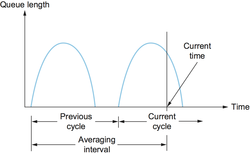
Figure 34. Computing average queue length at a router.

Now turning our attention to the host half of the mechanism, the source records how many of its packets resulted in some router setting the congestion bit. In particular, the source maintains a congestion window, just as in TCP, and watches to see what fraction of the last window’s worth of packets resulted in the bit being set. If less than 50% of the packets had the bit set, then the source increases its congestion window by one packet. If 50% or more of the last window’s worth of packets had the congestion bit set, then the source decreases its congestion window to 0.875 times the previous value. The value 50% was chosen as the threshold based on analysis that showed it to correspond to the peak of the power curve. The “increase by 1, decrease by 0.875” rule was selected because additive increase/multiplicative decrease makes the mechanism stable.

6.2 Random Early Detection

A second mechanism, called random early detection (RED), is similar to the DECbit scheme in that each router is programmed to monitor its own queue length and, when it detects that congestion is imminent, to notify the source to adjust its congestion window. RED, invented by Sally Floyd and Van Jacobson in the early 1990s, differs from the DECbit scheme in two major ways.

Further Reading

S. Floyd and V. Jacobson Random Early Detection (RED) Gateways for Congestion Avoidance. IEEE/ACM Transactions on Networking. August 1993.

The first is that rather than explicitly sending a congestion notification message to the source, RED is most commonly implemented such that it implicitly notifies the source of congestion by dropping one of its packets. The source is, therefore, effectively notified by the subsequent timeout or duplicate ACK. In case you haven’t already guessed, RED is designed to be used in conjunction with TCP, which currently detects congestion by means of timeouts (or some other means of detecting packet loss such as duplicate ACKs). As the “early” part of the RED acronym suggests, the gateway drops the packet earlier than it would have to, so as to notify the source that it should decrease its congestion window sooner than it would normally have. In other words, the router drops a few packets before it has exhausted its buffer space completely, so as to cause the source to slow down, with the hope that this will mean it does not have to drop lots of packets later on.

The second difference between RED and DECbit is in the details of how RED decides when to drop a packet and what packet it decides to drop. To understand the basic idea, consider a simple FIFO queue. Rather than wait for the queue to become completely full and then be forced to drop each arriving packet (the tail drop policy described in Section 2.1.3), we could decide to drop each arriving packet with some drop probability whenever the queue length exceeds some drop level. This idea is called early random drop. The RED algorithm defines the details of how to monitor the queue length and when to drop a packet.

In the following paragraphs, we describe the RED algorithm as originally proposed by Floyd and Jacobson. We note that several modifications have since been proposed both by the inventors and by other researchers. However, the key ideas are the same as those presented below, and most current implementations are close to the algorithm that follows.

First, RED computes an average queue length using a weighted running average similar to the one used in the original TCP timeout computation. That is, AvgLen is computed as

\[\mathsf{AvgLen = (1 - Weight)\ x\ AvgLen + Weight\ x\ SampleLen}\]

where 0 < Weight < 1 and SampleLen is the length of the queue when a sample measurement is made. In most software implementations, the queue length is measured every time a new packet arrives at the gateway. In hardware, it might be calculated at some fixed sampling interval.

The reason for using an average queue length rather than an instantaneous one is that it more accurately captures the notion of congestion. Because of the bursty nature of Internet traffic, queues can become full very quickly and then become empty again. If a queue is spending most of its time empty, then it’s probably not appropriate to conclude that the router is congested and to tell the hosts to slow down. Thus, the weighted running average calculation tries to detect long-lived congestion, as indicated in the right-hand portion of Figure 35, by filtering out short-term changes in the queue length. You can think of the running average as a low-pass filter, where Weight determines the time constant of the filter. The question of how we pick this time constant is discussed below.

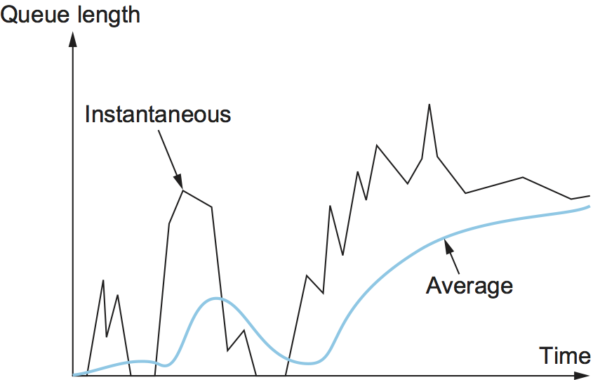
Figure 35. Weighted running average queue length.

Second, RED has two queue length thresholds that trigger certain activity: MinThreshold and MaxThreshold. When a packet arrives at the gateway, RED compares the current AvgLen with these two thresholds, according to the following rules:

if AvgLen <= MinThreshold 
    queue the packet 
if MinThreshold < AvgLen < MaxThreshold 
    calculate probability P 
    drop the arriving packet with probability P 
if MaxThreshold <= AvgLen 
    drop the arriving packet 

If the average queue length is smaller than the lower threshold, no action is taken, and if the average queue length is larger than the upper threshold, then the packet is always dropped. If the average queue length is between the two thresholds, then the newly arriving packet is dropped with some probability P. This situation is depicted in Figure 36. The approximate relationship between P and AvgLen is shown in Figure 37. Note that the probability of drop increases slowly when AvgLen is between the two thresholds, reaching MaxP at the upper threshold, at which point it jumps to unity. The rationale behind this is that, if AvgLen reaches the upper threshold, then the gentle approach (dropping a few packets) is not working and drastic measures are called for: dropping all arriving packets. Some research has suggested that a smoother transition from random dropping to complete dropping, rather than the discontinuous approach shown here, may be appropriate.

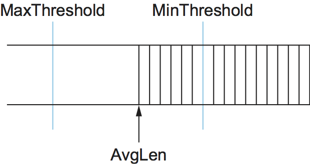
Figure 36. RED thresholds on a FIFO queue.

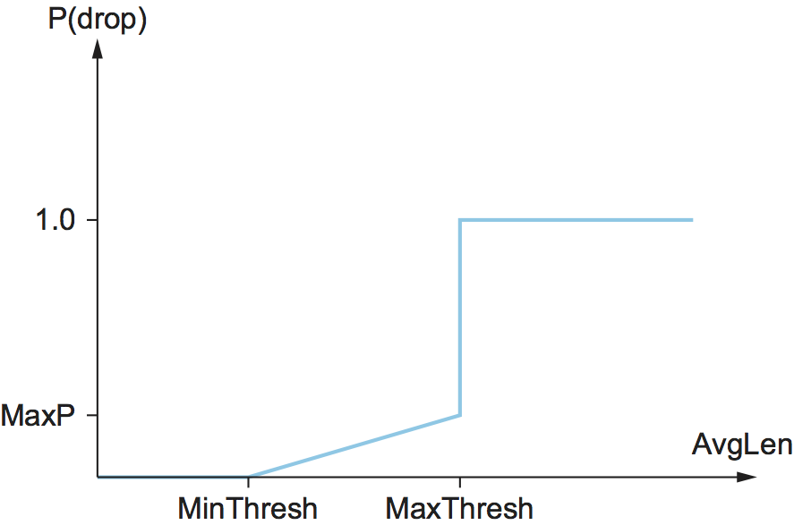
Figure 37. Drop probability function for RED.

Although Figure 37 shows the probability of drop as a function only of AvgLen, the situation is actually a little more complicated. In fact, P is a function of both AvgLen and how long it has been since the last packet was dropped. Specifically, it is computed as follows:

\[\mathsf{TempP = MaxP\ x\ (AvgLen - MinThreshold)\ /\ (MaxThreshold - MinThreshold)}\]

\[\mathsf{P = TempP\ /\ (1 - count\ x\ TempP)}\]

TempP is the variable that is plotted on the y-axis in Figure 37, count keeps track of how many newly arriving packets have been queued (not dropped), and AvgLen has been between the two thresholds. P increases slowly as count increases, thereby making a drop increasingly likely as the time since the last drop increases. This makes closely spaced drops relatively less likely than widely spaced drops. This extra step in calculating P was introduced by the inventors of RED when they observed that, without it, the packet drops were not well distributed in time but instead tended to occur in clusters. Because packet arrivals from a certain connection are likely to arrive in bursts, this clustering of drops is likely to cause multiple drops in a single connection. This is not desirable, since only one drop per round-trip time is enough to cause a connection to reduce its window size, whereas multiple drops might send it back into slow start.

As an example, suppose that we set MaxP to 0.02 and count is initialized to zero. If the average queue length were halfway between the two thresholds, then TempP, and the initial value of P, would be half of MaxP, or 0.01. An arriving packet, of course, has a 99 in 100 chance of getting into the queue at this point. With each successive packet that is not dropped, P slowly increases, and by the time 50 packets have arrived without a drop, P would have doubled to 0.02. In the unlikely event that 99 packets arrived without loss, P reaches 1, guaranteeing that the next packet is dropped. The important thing about this part of the algorithm is that it ensures a roughly even distribution of drops over time.

The intent is that, if RED drops a small percentage of packets when AvgLen exceeds MinThreshold, this will cause a few TCP connections to reduce their window sizes, which in turn will reduce the rate at which packets arrive at the router. All going well, AvgLen will then decrease and congestion is avoided. The queue length can be kept short, while throughput remains high since few packets are dropped.

Note that, because RED is operating on a queue length averaged over time, it is possible for the instantaneous queue length to be much longer than AvgLen. In this case, if a packet arrives and there is nowhere to put it, then it will have to be dropped. When this happens, RED is operating in tail drop mode. One of the goals of RED is to prevent tail drop behavior if possible.

The random nature of RED confers an interesting property on the algorithm. Because RED drops packets randomly, the probability that RED decides to drop a particular flow’s packet(s) is roughly proportional to the share of the bandwidth that flow is currently getting at that router. This is because a flow that is sending a relatively large number of packets is providing more candidates for random dropping. Thus, there is some sense of fair resource allocation built into RED, although it is by no means precise. While arguably fair, because RED punishes high-bandwidth flows more than low-bandwidth flows, it increases the probability of a TCP restart, which is doubly painful for those high-bandwidth flows.

A fair amount of analysis has gone into setting the various RED parameters—for example, MaxThreshold, MinThreshold, MaxP and Weight—all in the name of optimizing the power function (throughput-to-delay ratio). The performance of these parameters has also been confirmed through simulation, and the algorithm has been shown not to be overly sensitive to them. It is important to keep in mind, however, that all of this analysis and simulation hinges on a particular characterization of the network workload. The real contribution of RED is a mechanism by which the router can more accurately manage its queue length. Defining precisely what constitutes an optimal queue length depends on the traffic mix and is a subject of ongoing study.

Consider the setting of the two thresholds, MinThreshold and MaxThreshold. If the traffic is fairly bursty, then MinThreshold should be sufficiently large to allow the link utilization to be maintained at an acceptably high level. Also, the difference between the two thresholds should be larger than the typical increase in the calculated average queue length in one RTT. Setting MaxThreshold to twice MinThreshold seems to be a reasonable rule of thumb given the traffic mix on today’s Internet. In addition, since we expect the average queue length to hover between the two thresholds during periods of high load, there should be enough free buffer space above MaxThreshold to absorb the natural bursts that occur in Internet traffic without forcing the router to enter tail drop mode.

We noted above that Weight determines the time constant for the running average low-pass filter, and this gives us a clue as to how we might pick a suitable value for it. Recall that RED is trying to send signals to TCP flows by dropping packets during times of congestion. Suppose that a router drops a packet from some TCP connection and then immediately forwards some more packets from the same connection. When those packets arrive at the receiver, it starts sending duplicate ACKs to the sender. When the sender sees enough duplicate ACKs, it will reduce its window size. So, from the time the router drops a packet until the time when the same router starts to see some relief from the affected connection in terms of a reduced window size, at least one round-trip time must elapse for that connection. There is probably not much point in having the router respond to congestion on time scales much less than the round-trip time of the connections passing through it. As noted previously, 100 ms is not a bad estimate of average round-trip times in the Internet. Thus, Weight should be chosen such that changes in queue length over time scales much less than 100 ms are filtered out.

Since RED works by sending signals to TCP flows to tell them to slow down, you might wonder what would happen if those signals are ignored. This is often called the unresponsive flow problem. Unresponsive flows use more than their fair share of network resources and could cause congestive collapse if there were enough of them, just as in the days before TCP congestion control. Some queueing techniques, such as weighted fair queueing, could help with this problem by isolating certain classes of traffic from others. There was also discussion of creating a variant of RED that could drop more heavily from flows that are unresponsive to the initial hints that it sends. However this turns out to be challenging because it can be hard to distinguish between non-responsive behavior and "correct" behavior, especially when flows have a wide variety of different RTTs and bottleneck bandwidths.

As a footnote, 15 prominent network researchers urged for the widespread adoption of RED-inspired AQM in 1998. The recommendation was largely ignored, for reasons that we touch on below. AQM approaches based on RED have, however, been applied with some success in datacenters.

Further Reading

R. Braden, et al. Recommendations on Queue Management and Congestion Avoidance in the Internet. RFC 2309, April 1998.

6.3 Controlled Delay

As noted in the preceding section, RED has never been widely adopted. Certainly it never reached the level necessary to have a significant impact on congestion in the Internet. One reason is that RED is difficult to configure in a way that consistently improves performance. Note the large number of parameters that affect its operation (MinThreshold, MaxThreshold, and Weight). There is enough research showing that RED produces a wide range of outcomes (not all of them helpful) depending on the type of traffic and parameter settings. This created uncertainty around the merits of deploying it.

Over a period of years, Van Jacobson (well known for his work on TCP Congestion and a co-author of the original RED paper) collaborated with Kathy Nichols and eventually other researchers to come up with an AQM approach that improves upon RED. This work became known as CoDel (pronounced coddle) for Controlled Delay AQM. CoDel builds on several key insights that emerged over decades of experience with TCP and AQM.

Further Reading

K. Nichols and V. Jacobson. Controlling Queue Delay. ACM Queue, 10(5), May 2012.

First, queues are an important aspect of networking and it is expected that queues will build up from time to time. For example, a newly opened connection may dump a window’s worth of packets into the network, and these are likely to form a queue at the bottleneck link. This is not in itself a problem. There should be enough buffer capacity to absorb such bursts. Problems arise when there is not enough buffer capacity to absorb bursts, leading to excessive loss. This came to be understood in the 1990s as a requirement that buffers be able to hold at least one bandwidth-delay product of packets—a requirement that was probably too large and subsequently questioned by further research. But the fact is that buffers are necessary, and it is expected that they will be used to absorb bursts. The CoDel authors refer to this as "good queue", as illustrated in Figure 38 (a).

Figure 38. Good and Bad Queue Scenarios

Queues become a problem when they are persistently full. A persistently full queue is doing nothing except adding delay to the network, and it is also less able to absorb bursts if it never drains fully. The combination of large buffers and persistent queues within those buffers is a phenomenon that Jim Gettys has named Bufferbloat. It is clear that persistently full queues are what a well-designed AQM mechanism would seek to avoid. Queues that stay full for long periods without draining are referred to, unsurprisingly, as "bad queue", as shown in Figure 38 (b).

Further Reading

J. Gettys. Bufferbloat: Dark Buffers in the Internet. IEEE Internet Computing, April 2011.

In a sense, then, the challenge for an AQM algorithm is to distinguish between "good" and "bad" queues, and to trigger packet loss only when the queue is determined to be "bad". Indeed, this is what RED is trying to do with its weight parameter (which filters out transient queue length).

One of the innovations of CoDel is to focus on sojourn time: the time that any given packet waits in the queue. Sojourn time is independent of the bandwidth of a link and provides useful indication of congestion even on links whose bandwidth varies over time, such as wireless links. A queue that is behaving well will frequently drain to zero, and thus, some packets will experience a sojourn time close to zero, as in Figure 38 (a). Conversely, a congested queue will delay every packet, and the minimum sojourn time will never be close to zero, as seen in Figure 38 (b). CoDel therefore measures the sojourn time—something that is easy to do for every packet—and tracks whether it is consistently sitting above some small target. "Consistently" is defined as "lasting longer than a typical RTT".

Rather than asking operators to determine the parameters to make CoDel work well, the algorithm chooses reasonable defaults. A target sojourn time of 5ms is used, along with a sliding measurement window of 100ms. The intuition, as with RED, is that 100ms is a typical RTT for traffic traversing the Internet, and that if congestion is lasting longer than 100ms, we may be moving into the "bad queue" region. So CoDel monitors the sojourn time relative to the target of 5ms. If it is above target for more than 100ms, it is time to start taking action to reduce the queue via drops (or marking if explicit congestion notification, described below, is available). 5ms is chosen as being close to zero (for better delay) but not so small that the queue would run empty. It should be noted that a great deal of experimentation and simulation has gone into these numerical choices, but more importantly, the algorithm does not seem to be overly sensitive to them.

To summarize, CoDel largely ignore queues that last less than an RTT, but starts taking action as soon as a queue persists for more than an RTT. By making reasonable assumptions about Internet RTTs, the algorithm requires no configuration parameters.

An additional subtlety is that CoDel drops a slowly increasing percentage of traffic as long as the observed sojourn time remains above the target. As discussed further in Section 7.4, TCP throughput has been shown to depend inversely on the square root of loss rate. Thus, as long as the sojourn time stays above the target, CoDel steadily increases its drop rate in proportion to the square root of the number of drops since the target was exceeded. The effect of this, in theory, is to cause a linear decrease in throughput of the affected TCP connections. Eventually this should lead to enough reduction in arriving traffic to allow the queue to drain, bringing the sojourn time back below the target.

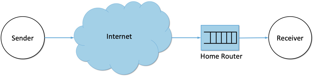
Figure 39. Home routers can suffer from bufferbloat, a situation CoDel is well-suited to address.

There are more details to CoDel presented in the Nichols and Jacobson paper, including extensive simulations to indicate its effectiveness across a wide range of scenarios. The algorithm has been standardized as "experimental" by the IETF in RFC 8289. It is also implemented in the Linux kernel, which has aided in its deployment. In particular, CoDel provides value in home routers (which are often Linux-based), a point along the end-to-end path (see Figure 39) that commonly experiences bufferbloat.

6.4 Explicit Congestion Notification

While TCP’s congestion control mechanism was initially based on packet loss as the primary congestion signal, it has long been recognized that TCP could do a better job if routers were to send a more explicit congestion signal. That is, instead of dropping a packet and assuming TCP will eventually notice (e.g., due to the arrival of a duplicate ACK), any AQM algorithm can potentially do a better job if it instead marks the packet and continues to send it along its way to the destination. This idea was codified in changes to the IP and TCP headers known as Explicit Congestion Notification (ECN), as specified in RFC 3168.

Further Reading

K. Ramakrishnan, S. Floyd, and D. Black. The Addition of Explicit Congestion Notification (ECN) to IP. RFC 3168, September 2001.

Specifically, this feedback is implemented by treating two bits in the IP TOS field as ECN bits. One bit is set by the source to indicate that it is ECN-capable, that is, able to react to a congestion notification. This is called the ECT bit (ECN-Capable Transport). The other bit is set by routers along the end-to-end path when congestion is encountered, as computed by whatever AQM algorithm it is running. This is called the CE bit (Congestion Encountered).

In addition to these two bits in the IP header (which are transport-agnostic), ECN also includes the addition of two optional flags to the TCP header. The first, ECE (ECN-Echo), communicates from the receiver to the sender that it has received a packet with the CE bit set. The second, CWR (Congestion Window Reduced) communicates from the sender to the receiver that it has reduced the congestion window.

While ECN is now the standard interpretation of two of the eight bits in the TOS field of the IP header and support for ECN is highly recommended, it is not required. Moreover, there is no single recommended AQM algorithm, but instead, there is a list of requirements a good AQM algorithm should meet. Like TCP congestion control algorithms, every AQM algorithm has its advantages and disadvantages, and so we need a lot of them to argue about.

6.5 Ingress/Egress Queues

We have been drawing a clear line between approaches to congestion control that happen inside the network (i.e., the AQM algorithms described in this chapter) and at the edge of the network (i.e., the TCP-based algorithms described in earlier chapters). But the line isn’t necessarily that crisp. To see this, you just have to think of the end-to-end path as having a ingress queue at the kernel/device interface on the sending host and an egress queue at the device/kernel interface on the receiving host.1 These edge queues are likely to become increasingly important as virtual switches and NIC support for virtualization become more and more common.

1

Confusingly, the ingress queue from the perspective of the network path is the outbound (egress) queue on the sending host and, the egress queue from the perspective of the network path is the inbound (ingress) queue on the receiving host. As shown in Figure 40, we use the terms ingress and egress from the network’s perspective.

This perspective is illustrated in Figure 40, where both locations sit below TCP, and provide an opportunity to inject a second piece of congestion control logic into the end-to-end path. CoDel and ECN are examples of this idea: they have been implemented at the device queue level of the Linux kernel.

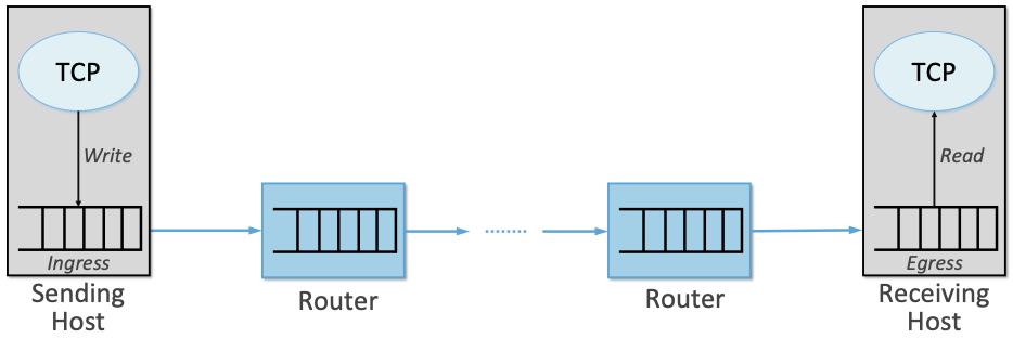
Figure 40. Ingress and egress queues along the end-to-end path, implemented in the sending and receiving hosts, respectively.

Does this work? One issue is whether packets are dropped at the ingress or the egress. When dropping at the ingress (on the sending host), TCP is notified in the return value of the Write function, which causes it to “forget” that it sent the packet. This means this packet will be sent next, although TCP does decrease its congestion window in response to the failed write. In contrast, dropping packets at the egress queue (on the receiving host), means the TCP sender will not know to retransmit the packet until it detects the loss using one of its standard mechanisms (e.g., three duplicate ACKs, a timeout). Of course, having the egress implement ECN helps.

When we consider this discussion in the context of the bigger congestion control picture, we can make two interesting observations. One is that Linux provides a convenient and safe way to inject new code—including congestion control logic—into the kernel, namely, using the extended Berkeley Packet Filter (eBPF). eBPF is becoming an important technology in many other contexts as well. The standard kernel API for congestion control has been ported to eBPF and most existing congestion control algorithms have been ported to this framework. This simplifies the task of experimenting with new algorithms or tweaking existing algorithms by side-stepping the hurdle of waiting for the relevant Linux kernel to be deployed.

Further Reading

The Linux Kernel. BPF Documentation.

A second observation is that by explicitly exposing the ingress/egress queues to the decision-making process, we open the door to building a congestion control mechanism that contains both a “decide when to transmit a packet” component and a “decide to queue-or-drop a packet” component. We’ll see an example of a mechanism that takes an innovative approach to using these two components in Section 7.1 when we describe On-Ramp.